MUMINS: Metadata-conditioned Uncertainty-aware Medical Image Next-state Synthesis
1Eurecat, Centre Tecnològic de Catalunya, Barcelona, Spain
2Dept. de Matemàtiques i Informàtica, Universitat de Barcelona, Spain
3Barcelona Supercomputing Center (BSC), Spain



A future scan, and a map of where it is uncertain.
From one baseline scan and a target time interval.
Forecasting change while preserving anatomy
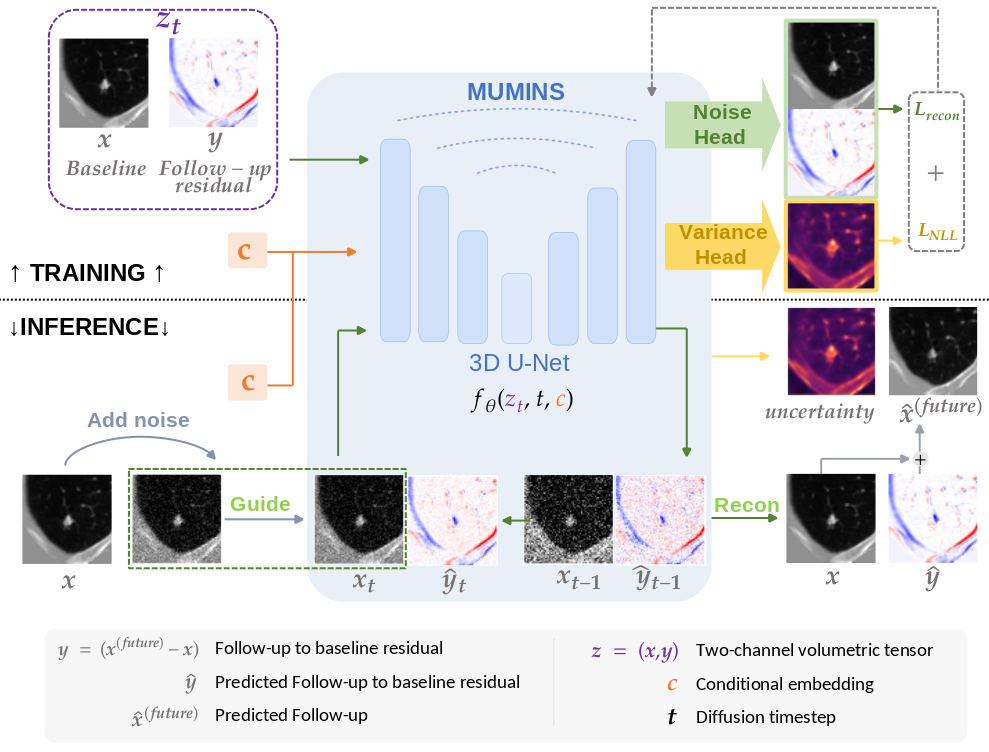
MUMINS models longitudinal change as a residual added to an observed baseline scan. A 3D diffusion model jointly learns the baseline and residual, conditioned on the follow-up interval, age, and acquisition metadata. During synthesis, the observed baseline is re-injected at every denoising step to keep the predicted change tied to the patient's anatomy.
One sampling process, two outputs
A learned variance head estimates uncertainty alongside each noise prediction. These estimates are propagated through the reverse process, producing a spatial uncertainty map together with the synthesized follow-up, without repeatedly sampling the model for Monte Carlo uncertainty.
- Joint baseline–residual diffusion separates relatively stable anatomy from the change to be synthesized.
- Temporal and metadata conditioning controls the follow-up horizon and accounts for age and acquisition-related sharpness changes.
- Baseline reinjection anchors the predicted residual to the observed scan throughout denoising.
- Single-pass uncertainty highlights regions where the synthesized follow-up is less reliable.
From pulmonary nodules to brain MRI
The same architecture is trained separately on two longitudinal datasets: PNG for pulmonary nodule progression in chest CT, and OASIS-3 for brain MRI progression. Each dataset has its own trained model; no organ-specific architectural components are introduced.

Quantitative synthesis results
The tables report whole-image means across all test pairs from Table 1 of the preprint, including both MUMINS blur-conditioning settings. Δb describes the change in acquisition blur between the baseline and follow-up scans.
- MUMINS (Δb = 0) preserves the baseline scan's sharpness and requires no information from the unseen follow-up. This is the deployable forecasting setting, used for comparison with methods that also lack access to the true follow-up.
- MUMINS (Δb = GT) uses the blur difference measured from the ground-truth follow-up. It is an oracle diagnostic upper bound: it requires the true follow-up, so it cannot be used to forecast an unseen scan.
Reporting both settings helps separate acquisition-related appearance changes from anatomical progression. The benchmark scans contain real changes in blur between visits: Δb = 0 preserves baseline sharpness, while Δb = GT accounts for that observed drift, improving agreement with the recorded follow-up. See Section 3.3 and Section 4.4 of the preprint.
| Method | MAE (×10⁻²) ↓ | PSNR (dB) ↑ | SSIM (%) ↑ |
|---|---|---|---|
| Copy baseline | 4.54 | 21.91 | 65.21 |
| GM-AE | 4.05 | 22.88 | 65.69 |
| TADM-3D | 4.91 | 21.39 | 66.77 |
| NGP-Net | 4.13 | 22.85 | 71.34 |
| MUMINS (Δb = 0) | 3.95 | 23.53 | 71.40 |
| MUMINS (Δb = GT, oracle) | 3.18 | 25.50 | 78.01 |
| Method | MAE (×10⁻²) ↓ | PSNR (dB) ↑ | SSIM (%) ↑ |
|---|---|---|---|
| Copy baseline | 1.14 | 30.91 | 95.55 |
| BrLP | 1.57 | 27.12 | 94.12 |
| TADM-3D | 1.21 | 30.12 | 94.99 |
| MUMINS (Δb = 0) | 1.13 | 30.87 | 95.34 |
| MUMINS (Δb = GT, oracle) | 1.05 | 31.35 | 95.64 |
Lower MAE and higher PSNR/SSIM are better. Bold values are the best across the listed rows, including the GT oracle setting. On brain MRI, copying the baseline is a strong reference because longitudinal changes are subtle. See Table 1 for standard deviations, subgroup results, and region-of-interest metrics.
Explore the predicted follow-up, slice by slice
Explore every slice in axial, coronal, and sagittal views. The lung CT example includes baseline, observed follow-up, prediction, uncertainty, and absolute error; the brain MRI example shows prediction and predicted uncertainty. Use the slider to choose a slice, or press Play to animate. Zoom is controlled only by the + and − buttons. Both examples use Δb = 0, preserving the baseline scan’s sharpness.
Lung CT · PNG
64 slices per plane · Full follow-up comparison
Compare the follow-up




Brain MRI · OASIS-3
128 slices per plane · Prediction and uncertainty
Prediction & uncertainty
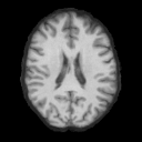
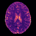
Ground-truth (GT) OASIS-3 scans are omitted from this interactive viewer because the dataset's data-use agreement restricts redistribution. Only MUMINS predictions and predicted uncertainty are shown.
The animation moves through spatial slices at a fixed follow-up interval. Uncertainty σ is predicted standard deviation; absolute error compares the prediction with the true follow-up. Color scales use normalized intensity units and remain fixed across slices within each modality; values outside the displayed limits are clipped.
Where is the predicted follow-up uncertain?
Compare the observed baseline, actual follow-up, synthesized follow-up, learned uncertainty, and absolute error on held-out examples. Brighter uncertainty regions indicate greater predicted uncertainty; absolute error is computed against the observed follow-up.
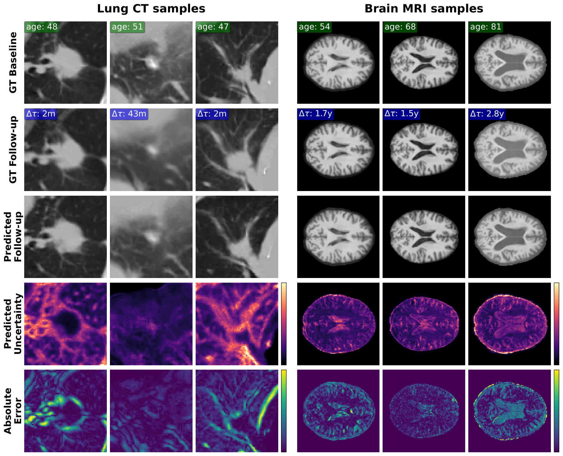
The uncertainty map is evaluated against true voxel-wise error, rather than treating Monte Carlo variation as ground truth. Whole-image Spearman correlations are 0.61 for lung CT and 0.54 for brain MRI. Nominal 95% interval coverage is 0.91 and 0.98, respectively. See Table 2 for calibration, region-of-interest results, and the 20-sample Monte Carlo comparison.
Code and reproducibility
The official PyTorch implementation includes dataset preparation guidance, training configurations, and inference scripts for follow-up volumes and uncertainty maps. The repository also documents the OASIS-3 sample selection used in the experiments.
Cite
Accepted to WACV 2027. The citation below refers to the arXiv preprint.
@misc{oliveras2026mumins,
  title         = {MUMINS: Metadata-conditioned Uncertainty-aware Medical Image Next-state Synthesis},
  author        = {Anna Oliveras and Roger Marí and Rafael Redondo and Oriol Guardià-Olivella and Cynthia Ifeyinwa Ugwu and Ana Tost and Bhalaji Nagarajan and Carolina Migliorelli and Vicent Ribas and Petia Radeva},
  year          = {2026},
  eprint        = {2609.17169},
  archivePrefix = {arXiv},
  primaryClass  = {cs.CV},
  url           = {https://arxiv.org/abs/2609.17169}
}
Acknowledgments and funding
A. Oliveras acknowledges Eurecat’s “Vicente López” PhD grant program. This work was supported by computational resources provided by Finis Terrae III (CESGA) and the Barcelona Supercomputing Center (BCV-2026-2-0027), and by the PHASE IV AI project, funded by the European Union under the Horizon Europe grant agreement No. 101095384.
This work was partially funded by Icrea Academia’2022 (Generalitat de Catalunya), IDEATE (PID2022-141566NB-I00) and TRI-VISION (PID2025-173459NB-C21) both funded by MICIU/AEI/10.13039/501100011033 and by FEDER/EU, and EXPLORA-SCALE (AIA2025-163919-C51) funded by MICIU/AEI/10.13039/501100011033.
B. Nagarajan acknowledges AI4S fellowship within the “Generación D” initiative by Red.es, Ministerio para la Transformación Digital y de la Función Pública, for talent attraction (C005/24-ED CV1), funded by NextGenerationEU through PRTR.